Program description
boundfit determines upper and lower boundaries to a given data set using the generalised least-squares method described in Data boundary fitting using a generalised least-squares method (Cardiel 2009, MNRAS, 396, 680).
The key ideas behind this method are the following:
The sought boundary is iteratively determined starting from an initial guess fit. Ordinary least-squares fits provide suitable starting points. At every iteration in the procedure a particular fit is always available.
In each iteration the data to be fitted are segregated in two subgroups depending on their position relative to the particular fit at that iteration. In this sense, points are classified as being inside or outside of the boundary.
Points located outside of the boundary are given an extra weight in the cost function to be minimised. This weight is parametrized through the asymmetry coefficient, which net effect is to generate a stronger pulling effect of the outer points over the fit, which in this way shifts towards the frontier delineated by the outer points as the iterations proceed.
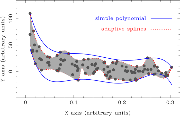
The minimisation of the cost function can be easily carried out using the popular DOWNHILL simplex method. In principle this allows the use of any complutable function as the analytical expression for the boundary fits. boundfit incorporates the use of simple polynomials and adaptive splines as the two possible functional forms for the computed boundaries.
In the general case, given a set of  data points
  ,
with optional
,
with optional  uncertainties associated to the
  data, the boundary to be fitted will be a function depending on
  parameters
  , which values will be obtained by
the minimisation of
, which values will be obtained by
the minimisation of
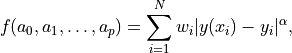
where  is the boundary function evaluated at
  , and
, and
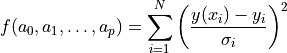
For the particular case  ,
,  , and
, and
 one gets the traditional cost function for the ordinary
least-squares fit
one gets the traditional cost function for the ordinary
least-squares fit
The new method includes a set of tunable parameters  and
and  , which roles are basically the following:
 : the power that controls how distances between the data points
and the boundary fit are computed. Since this number its a real number, the
difference
: the power that controls how distances between the data points
and the boundary fit are computed. Since this number its a real number, the
difference  must be introduced in the first expression in
absolute value.
must be introduced in the first expression in
absolute value. : the power for the error weighting. It has been defined as an
additional parameter to have the possibility of using a value different from
(which in ordinary least-squares is set to 2).
: the power for the error weighting. It has been defined as an
additional parameter to have the possibility of using a value different from
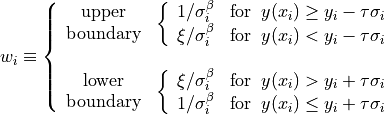
(which in ordinary least-squares is set to 2).- : this is the asymmetry coefficient, which is responsible for
giving a different weight to the data points at both sides (inside and
outside) of the boundary being fitted. For the method to work properly, a
value of
 must be employed.
  : cut-off parameter that allows some points to be left outside of
the boundary fit. Since this parameter is used together with the data
uncertainties σi, its use help to perform the computation of a boundary fit
leaving the points with larger errors outside of the boundary.
: cut-off parameter that allows some points to be left outside of
the boundary fit. Since this parameter is used together with the data
uncertainties σi, its use help to perform the computation of a boundary fit
leaving the points with larger errors outside of the boundary.
A much more detailed description of this method, and the parameters
(, , and ) that can be tuned
to modify the behaviour of the fitting procedure depending on the nature of the
data being fitted, is given in Cardiel2009.
Example
The fits displayed in the following figure (Figure 6 from Cardiel2009) have been
computed using option 1 “Simple polynomial (generic version)” and option 3
“Adaptive splines”, which are explained below. The data points are those given
in the file example.dat.
The following shell scripts can be used to reproduce the plotted boundary fits:
type of fit |
boundary |
script |
|---|---|---|
simple polynomial (generic version) |
upper boundary |
|
simple polynomial (generic version) |
lower boundary |
|
adaptive splines |
upper boundary |
|
adaptive splines |
lower boundary |
Each of the different scriptj.csh/.sh files (with j=1, 2, 3 or 4) reads the ascii input file example.dat and generates an ascii output file called scriptj.out containing a collection of 1000 points defining the corresponding boundary data.